
Notice
Recent Posts
Recent Comments
Link
250x250
| 일 | 월 | 화 | 수 | 목 | 금 | 토 |
|---|---|---|---|---|---|---|
| 1 | 2 | 3 | 4 | 5 | 6 | 7 |
| 8 | 9 | 10 | 11 | 12 | 13 | 14 |
| 15 | 16 | 17 | 18 | 19 | 20 | 21 |
| 22 | 23 | 24 | 25 | 26 | 27 | 28 |
Tags
- 데이터 구축
- RNN
- ODQA
- nlp
- passage retrieval
- Bert
- word2vec
- mrc
- AI 경진대회
- Data Viz
- seaborn
- 기아
- N21
- 딥러닝
- N2N
- Attention
- Ai
- AI Math
- Transformer
- KLUE
- Optimization
- 현대자동차
- pyTorch
- dataset
- Self-attention
- Bart
- 2023 현대차·기아 CTO AI 경진대회
- GPT
- matplotlib
- 데이터 시각화
Archives
- Today
- Total
쉬엄쉬엄블로그
(Data Viz) Seaborn 기초 실습 - 4 (Relational API, Regression API) 본문
부스트캠프 AI Tech 4기
(Data Viz) Seaborn 기초 실습 - 4 (Relational API, Regression API)
쉬엄쉬엄블로그 2023. 6. 28. 11:40728x90
이 색깔은 주석이라 무시하셔도 됩니다.
Seaborn 기초 실습
기본적인 분류 5가지의 기본적인 종류의 통계 시각화와 형태 살펴보기
- Categorical API
- Distribution API
- Relational API
- Regression API
- Matrix API
라이브러리와 데이터셋 호출
import numpy as np
import pandas as pd
import matplotlib as mpl
import matplotlib.pyplot as plt
import seaborn as sns

print('seaborn version : ', sns.__version__)

"""
seaborn version :  0.11.2
"""
student = pd.read_csv('./StudentsPerformance.csv')
student.head()
4. Relation & Regression API
4-1. Scatter Plot
산점도는 다음과 같은 요소를 사용할 수 있다.
stylehuesize
style, hue, size에 대한 순서는 각각 style_order, hue_order, size_order로 전달할 수 있다.
fig, ax = plt.subplots(figsize=(7, 7))
sns.scatterplot(x='math score', y='reading score', data=student,
#                style='gender', markers={'male':'s', 'female':'o'},
                hue='race/ethnicity',
#                 size='writing score',
               )
plt.show()
4-2. Line Plot
시계열 데이터 시각화
flights = sns.load_dataset("flights")
flights.head()
flights_wide = flights.pivot("year", "month", "passengers")
flights_wide.head()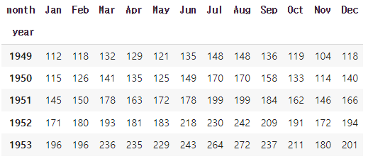
fig, ax = plt.subplots(1, 1,figsize=(12, 7))
sns.lineplot(x='year', y='Jan',data=flights_wide, ax=ax)
fig, ax = plt.subplots(1, 1,figsize=(12, 7))
sns.lineplot(data=flights_wide, ax=ax)
plt.show()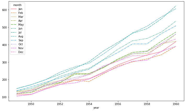
자동으로 평균과 표준편차로 오차범위를 시각화해준다.
fig, ax = plt.subplots(1, 1, figsize=(12, 7))
sns.lineplot(data=flights, x="year", y="passengers", ax=ax)
plt.show()
fig, ax = plt.subplots(1, 1, figsize=(12, 7))
sns.lineplot(data=flights, x="year", y="passengers", hue='month',
             style='month', markers=True, dashes=False,
             ax=ax)
plt.show()
4-3. Regplot
회귀선을 추가한 scatter plot
fig, ax = plt.subplots(figsize=(7, 7))
sns.regplot(x='math score', y='reading score', data=student,
               )
plt.show()
한 축에 한 개의 값만 보여주기 위해서 다음과 같이 사용할 수 있다.
fig, ax = plt.subplots(figsize=(7, 7))
sns.regplot(x='math score', y='reading score', data=student,
            x_estimator=np.mean
           )
plt.show()
보여주는 개수도 지정할 수 있다.
fig, ax = plt.subplots(figsize=(7, 7))
sns.regplot(x='math score', y='reading score', data=student,
            x_estimator=np.mean, x_bins=20
           )
plt.show()
다차원 회귀선은 order 파라미터를 통해 전달할 수 있다.
다만 현재 데이터에서는 선형성이 강해 따로 2차원으로 회귀선을 그리지 않아도 잘 보이는 것을 알 수 있다.
fig, ax = plt.subplots(figsize=(7, 7))
sns.regplot(x='math score', y='reading score', data=student,
            order=2
           )
plt.show()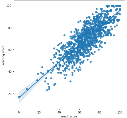
로그를 사용할 수도 있다.
fig, ax = plt.subplots(figsize=(7, 7))
sns.regplot(x='reading score', y='writing score', data=student,
            logx=True
           )
plt.show()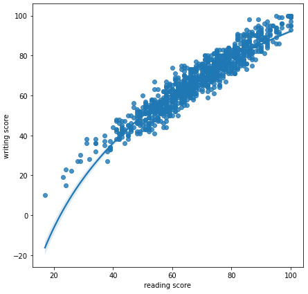
출처: 부스트캠프 AI Tech 4기(NAVER Connect Foundation)
'부스트캠프 AI Tech 4기' 카테고리의 다른 글
| (Data Viz) Polar Coordinate - Polar Plot (0) | 2023.06.30 |
|---|---|
| (Data Viz) Seaborn 기초 실습 - 5 (Matrix API) (2) | 2023.06.29 |
| (Data Viz) Seaborn 기초 실습 - 3 (Distribution API) (0) | 2023.06.27 |
| (Data Viz) Seaborn 기초 실습 - 2 (Categorical API) (0) | 2023.06.24 |
| (Data Viz) Seaborn 기초 실습 - 1 (0) | 2023.06.24 |
'부스트캠프 AI Tech 4기' Related Articles
more


Comments