
Notice
Recent Posts
Recent Comments
Link
250x250
| 일 | 월 | 화 | 수 | 목 | 금 | 토 |
|---|---|---|---|---|---|---|
| 1 | 2 | 3 | 4 | 5 | 6 | 7 |
| 8 | 9 | 10 | 11 | 12 | 13 | 14 |
| 15 | 16 | 17 | 18 | 19 | 20 | 21 |
| 22 | 23 | 24 | 25 | 26 | 27 | 28 |
Tags
- KLUE
- 데이터 구축
- Bart
- 데이터 시각화
- Transformer
- Self-attention
- N2N
- 기아
- RNN
- word2vec
- pyTorch
- AI Math
- passage retrieval
- nlp
- Attention
- 2023 현대차·기아 CTO AI 경진대회
- mrc
- Bert
- Data Viz
- Ai
- GPT
- matplotlib
- seaborn
- 현대자동차
- 딥러닝
- AI 경진대회
- N21
- Optimization
- ODQA
- dataset
Archives
- Today
- Total
쉬엄쉬엄블로그
(Data Viz) Seaborn 기초 실습 - 3 (Distribution API) 본문
728x90
이 색깔은 주석이라 무시하셔도 됩니다.
Seaborn 기초 실습
기본적인 분류 5가지의 기본적인 종류의 통계 시각화와 형태 살펴보기
- Categorical API
- Distribution API
- Relational API
- Regression API
- Matrix API
라이브러리와 데이터셋 호출
import numpy as np
import pandas as pd
import matplotlib as mpl
import matplotlib.pyplot as plt
import seaborn as sns

print('seaborn version : ', sns.__version__)

"""
seaborn version :  0.11.2
"""
student = pd.read_csv('./StudentsPerformance.csv')
student.head()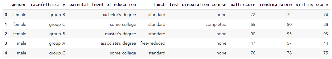
3. Distribution API
범주형/연속형을 모두 살펴볼 수 있는 분포 시각화를 살펴본다.
3-1. Univariate Distribution
histplot: 히스토그램kdeplot: Kernel Density Estimateecdfplot: 누적 밀도 함수rugplot: 선을 사용한 밀도함수
fig, axes = plt.subplots(2,2, figsize=(12, 10))
axes = axes.flatten()

sns.histplot(x='math score', data=student, ax=axes[0])

sns.kdeplot(x='math score', data=student, ax=axes[1])

sns.ecdfplot(x='math score', data=student, ax=axes[2])

sns.rugplot(x='math score', data=student, ax=axes[3])


plt.show()
histplot (히스토그램)
막대 개수나 간격에 대한 조정은 대표적으로 2가지 파라미터가 있다.
binwidthbins
fig, ax = plt.subplots(figsize=(12, 7))

sns.histplot(x='math score', data=student, ax=ax,
#              binwidth=50,
#              bins=100,
            )

plt.show()
히스토그램은 기본적으로 막대지만, seaborn에서는 다른 표현들도 제공하고 있다.
fig, ax = plt.subplots(figsize=(12, 7))

sns.histplot(x='math score', data=student, ax=ax,
             element='poly' # step, poly
            )

plt.show()
히스토그램은 다음과 같이 N개의 분포를 표현할 수 있다.
fig, ax = plt.subplots(figsize=(12, 7))

sns.histplot(x='math score', data=student, ax=ax,
             hue='gender',
             multiple='stack', # layer, dodge, stack, fill
            )

plt.show()
kdeplot
연속확률밀도를 보여주는 함수로 seaborn의 다양한 smoothing 및 분포 시각화에 보조 정보로도 많이 사용한다.
fig, ax = plt.subplots(figsize=(12, 7))
sns.kdeplot(x='math score', data=student, ax=ax)
plt.show()
밀도 함수를 그릴 때는 단순히 선만 그려서는 정보의 전달이 어려울 수 있다.
fill='True'를 전달하여 내부를 채워 표현하는 것을 추천한다.

bw_method를 사용하여 분포를 더 자세하게 표현할 수도 있다.
fig, ax = plt.subplots(figsize=(12, 7))
sns.kdeplot(x='math score', data=student, ax=ax,
           fill=True, bw_method=0.05)
plt.show()
다양한 분포를 살펴본다. histogram의 연속적 표현이라고 생각하면 편하다.
fig, ax = plt.subplots(figsize=(12, 7))
sns.kdeplot(x='math score', data=student, ax=ax,
            fill=True,
            hue='race/ethnicity',
            hue_order=sorted(student['race/ethnicity'].unique()))
plt.show()
여러 분포를 표현하기 위해 다음과 같은 방법을 사용할 수 있다
stacklayerfill
fig, ax = plt.subplots(figsize=(12, 7))
sns.kdeplot(x='math score', data=student, ax=ax,
            fill=True,
            hue='race/ethnicity',
            hue_order=sorted(student['race/ethnicity'].unique()),
            multiple="layer", # layer, stack, fill
            cumulative=True,
            cut=0
           )
plt.show()
ecdfplot은 누적되는 양을 표현한다.
fig, ax = plt.subplots(figsize=(12, 7))
sns.ecdfplot(x='math score', data=student, ax=ax,
             hue='gender',
             stat='count', # proportion, count
             complementary=True
            )
plt.show()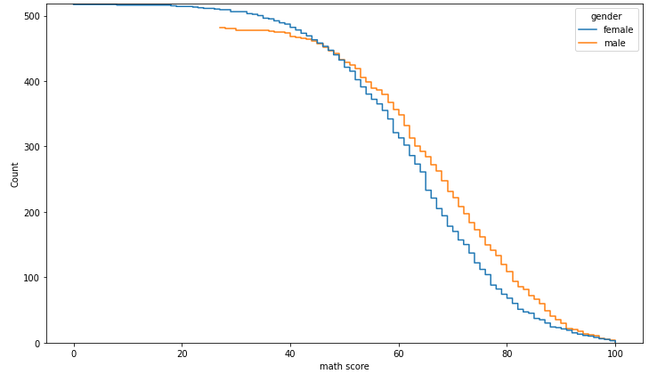
rugplot은 조밀한 정도를 통해 밀도를 나타낸다.
한정된 공간 내에서 분포를 표현하기에 좋은 것 같다.
fig, ax = plt.subplots(figsize=(12, 7))
sns.rugplot(x='math score', data=student, ax=ax)
plt.show()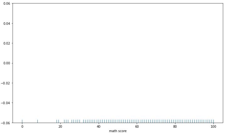
3-2. Bivariate Distribution
이제는 2개 이상 변수를 동시에 분포를 살펴본다.
결합 확률 분포(joint probability distribution)를 살펴 볼 수 있다.
함수는 histplot과 kdeplot을 사용하고, 입력에 1개의 축만 넣는 게 아닌 2개의 축 모두 입력을 넣어주는 것이 특징이다.
fig, axes = plt.subplots(1,2, figsize=(12, 7))
ax.set_aspect(1)

axes[0].scatter(student['math score'], student['reading score'], alpha=0.2)

sns.histplot(x='math score', y='reading score',
             data=student, ax=axes[1],
#              color='orange',
             cbar=False,
             bins=(10, 20),
            )

plt.show()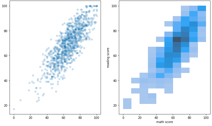
fig, ax = plt.subplots(figsize=(7, 7))
ax.set_aspect(1)

sns.kdeplot(x='math score', y='reading score',
             data=student, ax=ax,
            fill=True,
#             bw_method=0.1
            )

plt.show()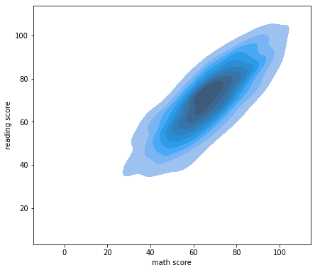
출처: 부스트캠프 AI Tech 4기(NAVER Connect Foundation)
'부스트캠프 AI Tech 4기' 카테고리의 다른 글
| (Data Viz) Seaborn 기초 실습 - 5 (Matrix API) (2) | 2023.06.29 |
|---|---|
| (Data Viz) Seaborn 기초 실습 - 4 (Relational API, Regression API) (0) | 2023.06.28 |
| (Data Viz) Seaborn 기초 실습 - 2 (Categorical API) (0) | 2023.06.24 |
| (Data Viz) Seaborn 기초 실습 - 1 (0) | 2023.06.24 |
| (Data Viz) Seaborn 소개 (0) | 2023.06.24 |
'부스트캠프 AI Tech 4기' Related Articles
more


Comments